Filter data by list conditions. Filtering data in the list. Filter using data form
Goal of the work: performing data sorting, familiarizing yourself with the method of filtering list entries, autofiltering, and working with data forms.
Exercise 1.
Sort the data in Table 5.5 several times in accordance with the following criteria - in alphabetical order of buyers' surnames, in descending order of transaction amount, in ascending order of transaction date, in combination of characteristics (last name, date, amount).
Method of doing the work
1. Open a new workbook and save it as “Sort” in your working folder .
2. Create the table shown in Figure 5.56.
Figure 5.56 – Initial table with data
3. Set formatting options for the table.
Font Times New Roman, font size 12 pt., for headings, bold style and center alignment, word wrapping, gray fill; for the main part. As a reminder, formatting commands are available on the Ribbon Home Þ Cells .
4. To sort by the buyer’s last name field, place the cursor anywhere in this column and run the command Data Þ Sorting (Fig. 5.51) .
In the dialog box that opens, in the field Sort by Select Buyer's Last Name. Ascending.
5. Repeat all the steps in step 4 and set the sorting by “Transaction Amount”, in descending order.
6. Re-sort by the “Transaction Date” field, ascending.
7. Copy the table to new leaf and sort on it by a set of characteristics. To do this, call the command Data Þ Sorting. Install Sort by surnames in ascending order, Then by date in ascending order, Lastly, by amount in descending order.
8. Using a command Rename Give names to these two sheets.
Task 2. Select information from the list based on the AutoFilter command.
Method of doing the work.
1. On sheet 4, create a table and fill it with information from table 5.5.
2. Rename Sheet4, giving it the name “AutoFilter #1”.
3. To apply AutoFiltering, place the cursor in the list area and run the command Data ÞFilter. Downward arrows will appear next to the names of the table columns, revealing a list of possible values. In the “Gender” column, select “M”. Copy the table to sheet 5 and rename it “Autofilter No. 2”.
4. On the “Autofilter No. 1” sheet, in the “Gender” column, open the filtering list and select “All”. Then, in the “Date of Birth” column, select “Condition” from the filtering list and set the condition (Fig. 5.57):
Table 5.5
| Surname | Name | employment date | Date of Birth | Floor | Salary | Age |
| Pashkov | Igor | 16.05.74 | 15.03.49 | M | ||
| Andreeva | Anna | 16.01.93 | 19.10.66 | AND | ||
| Erokhin | Vladimir | 23.10.81 | 24.04.51 | M | ||
| Popov | Alexei | 02.05.84 | 07.10.56 | M | ||
| Tyunkov | Vladimir | 03.11.88 | 19.07.41 | M | ||
| Notkin | Eugene | 27.08.85 | 17.08.60 | M | ||
| Kubrina | Marina | 20.04.93 | 26.06.61 | AND | ||
| Gudkov | Nikita | 18.03.98 | 05.04.58 | M | ||
| Gorbatov | Michael | 09.08.99 | 15.09.52 | M | ||
| Bystrov | Alexei | 06.12.00 | 08.10.47 | M | ||
| Krylova | Tatiana | 28.12.93 | 22.03.68 | AND | ||
| Bersheva | Olga | 14.12.01 | 22.12.74 | AND | ||
| Rusanova | Hope | 24.05.87 | 22.01.54 | AND |

Figure 5.57 – Setting filtering conditions
5. Copy the filtered table to sheet 6 and rename it “Autofilter No. 3. On the AutoFilter No. 1 sheet, deselect.

Figure 5.58 – Custom filter
6. In the “Last Name” column, select “Condition” in the filtering list and set a condition for selecting all employees whose last name begins with “B” (Fig. 5.58).
7. Copy the filtered list to sheet 7 and rename it “Autofilter No. 4”.
8. On the sheet “Autofilter No. 1” for the column “Last name” set “All”, and in the column “Salary” set “First 10...” where in the dialog box enter “Show the 5 largest elements of the list”.
9. Save the file.
Task 3. Select records from the list using the Advanced filter command.
Methodology for performing the work.
1. Go to Sheet 8 and rename it "Advanced Filter".
2. Copy the table from the previous task (Table 5.5) onto this sheet, paste it starting from line 7. The first 6 lines are reserved for setting conditions.
3. Let's create a range of conditions. Suppose we need to select the names of employees who earn more than 5,000 rubles. Or whose age exceeds 50 years. Fill in the conditions as shown in Figure 5.59.

Figure 5.59 – Conditions for an advanced filter
4. Run the command Data Þ Additional . Fill out the dialog box as follows (Fig. 5.60):

Figure 5.60 – Advanced filter parameters window
View the selection results. When writing conditions on one line, logical AND is implemented. When writing conditions on different lines, they are considered connected by logical OR. We have considered the first option, now we will consider the second.
5. Suppose we need to display only those employees whose last names begin with the letters A, G or N. Fill in the range of conditions (Figure 5.61).

Figure 5.61 – Conditions for an advanced filter
6. Run the command DataÞAdditional and fill out the dialog box (Figure 5.62).

Figure 5.62 – Advanced filter parameters window
View the results of the selection of records.
1. List all employees wage which are more than average. Before creating this filter, enter the formula =AVERAGE(F8:F20) in cell H2 to calculate the average salary.
2. Then in cell A2 we enter the calculated condition =F8>$H$2, which refers to cell H2 (Figures 5.63 and 5.64).

Figure 5.63 – Conditions for an advanced filter

Figure 5.64 – Advanced filter parameters
A filter is a quick and easy way to find a subset of data and work with it in a list. The filtered list displays only rows that meet the criteria. Unlike sorting, a filter does not change the order of entries in the list. Filtering temporarily hides rows that you don't want to display.
Rows selected by filtering can be edited, formatted, created into charts, and printed without changing the row order or moving them.
Filtering selects only the necessary data and hides the remaining data. This way, only what you want to see is shown, and it can be done with one click.
When filtering, the data does not change in any way. Once the filter is removed, all data appears again in the same form as it was before the filter was applied.
There are two commands available in Excel for filtering lists:
- Autofilter, including filter by selection, for simple conditions selection.
- Advanced filter for more difficult conditions selection.
Autofilter
To enable Autofilter you need to select any cell in the table, then on the tab Data in Group Sorting And filter press the big button :
After this, a down arrow button will appear in the table header to the right of each column heading:
Clicking an arrow opens a list menu for the corresponding column. The list contains all the elements of a column in alphabetical or numeric order (depending on the data type), so you can quickly find the element you need:

If we need a filter for only one column, then we don’t have to display arrow buttons for the remaining columns. To do this, before pressing the button select several cells of the desired column along with the heading.
Filter by exact value
Turn on Autofilter, click on the arrow button and select a value from the drop-down list. To quickly select all elements of a column or deselect all elements, click on the item (Select all) :

In this case, all rows whose field does not contain the selected value are hidden.
By doing laboratory work, select the filtering result, copy it to another place on the sheet and sign it.
To turn off Autofilter you need to press the button again .
To cancel the filter action without leaving the filtering mode, click on the button and select the item from the drop-down list (Select all) . In this case, table rows hidden by the filter appear.
Signs of data filtering
Filters hide data. This is exactly what they are designed for. However, if data filtering is not known, it may appear that some data is missing. You might, for example, open someone else's filtered sheet, or even forget that you yourself previously applied a filter. So when you have filters on a sheet, you can find different visual cues and messages.
(located at the bottom left of the window). The initial state:
![]()
Immediately after filtering the data, the result of applying the filter is displayed in the lower left corner of the status bar. For example, " Records found: 2 of 11”:
![]()
Line numbers . The broken line numbers indicate that some lines are hidden, and the changed color of the numbers visible lines indicates that the selected rows are the result of a filter selection.
Arrow type . When the AutoFilter arrow in a filtered column changes to, it indicates that the column is filtered.
”
“” is another universal filter that can be applied to columns with numbers or dates.
“” is a very conventional name. In fact, the capabilities of this filter are much wider. Using this filter, you can find either the first elements or the last elements (smallest or largest numbers or dates). And, contrary to the filter's name, the results obtained are not limited to the first 10 elements or the last 10 elements. The number of items displayed can be selected from 1 to 500.
” also allows you to filter data by percentage of the total number of rows in a column. If a column contains 100 numbers and you want to view the largest fifteen, then select 15 percent.
You can use the filter to find products with the highest or lowest prices, to determine the list of employees most recently hired, or to view a list of students with the best or worst grades. To apply the “” filter to a data column ( only numbers or dates!!!), click the arrow in the column and select the item Numeric filters Further :

After this, a dialog box will open Overlay conditions By list :

In the dialog box select number(rows or percentages), largest or smallest, list elements or % of the number of elements.
Create your own custom filters
For example, we need to output only rows with positions starting with the letter ‘ D’. To do this, click on the autofilter arrow in the first column and select Text filters , then point begin with… :

A dialog box will appear (Whichever item on the right you select, the same dialog box will still appear.):

In field Job title choose - begin with , on the right we enter d:

In the window there is a hint:
Question mark " ? ” means any one character.
Sign " * ” denotes a sequence of any characters.
You can select the necessary data from the list using filtering, that is, by hiding all rows of the list except those that meet the specified criteria. To use the filtering function, you need to place the table cursor on one of the list header cells (in our table this is the range A1:U11) and call the command Data/Filter/AutoFilter. Once activated, a small square with a drop-down arrow will appear in the lower right corner of each header cell.
Let's look at how to work with an autofilter using the following example. Let's determine how many representatives of the stronger sex work at the enterprise. Click the filter button located in the cell with the heading Gender, and select the letter M (male) from the list that opens. The message Filter: selection will appear in the status bar (Fig. 4.20). All rows that do not meet the specified criteria will be hidden. The arrow on the list button will turn blue to indicate that of this field Autofilter is enabled.
Rice. 4.20. Using an autofilter to select records based on "M" (male)
If you want to clarify how many of these men are bosses, also click the auto-filter button in the Position cell and select the word Chief in the corresponding list. A message will appear in the status bar indicating how many rows satisfy the specified criterion: Records found: 2 out of 10 (that is, the answer will be given immediately). The result is shown in Fig. 4.21.
To cancel filtering by a specific column, just open the AutoFilter list in that column and select All. However, if the filtering function is set on multiple columns, you will have to repeat this operation several times. In this case it is better to use the command Data/Filter/Display all.

Rice. 4.21. Worksheet after filtering the list of employees by the criterion “male boss”
The filtering function will work properly if you are careful when entering data. In particular, you need to ensure that there are no extra spaces at the beginning and end of the text data. They are not noticeable on the screen, but can lead to erroneous results, and a lot of time is spent identifying them.
Filtering selects data that exactly meets a given criterion. Therefore, if instead of the word "Head" the word "Head_" appears in a column, that is, with a space at the end, Excel treats these values as different. To get rid of inconsistencies of this kind, copy the cell with the word “Boss” to the clipboard, activate the filter for selecting by “Boss_” and replace the incorrect values with the contents of the buffer.
You can display information on one/several parameters using data filtering in Excel.
There are two tools for this purpose: AutoFilter and Advanced Filter. They do not delete, but hide data that does not meet the conditions. Autofilter performs the simplest operations. The advanced filter has much more options.
AutoFilter and Advanced Filter in Excel
I have a simple table that is not formatted or declared as a list. You can enable the automatic filter through the main menu.

If you format the data range as a table or declare it as a list, the automatic filter will be added immediately.
Using an autofilter is simple: you need to select the entry with the desired value. For example, display deliveries to store No. 4. Place a check mark next to the corresponding filtering condition:

We immediately see the result:
Features of the tool:
- The autofilter only works in a non-breaking range. Different tables on the same sheet are not filtered. Even if they have the same type of data.
- The tool treats the top line as column headings - these values are not included in the filter.
- It is permissible to apply several filtering conditions at once. But each previous result may hide the records needed for the next filter.
The advanced filter has much more options:
- You can set as many filtering conditions as needed.
- The criteria for selecting data are visible.
- Using the advanced filter, the user can easily find unique values in a multi-line array.
How to make an advanced filter in Excel
A ready-made example - how to use an advanced filter in Excel:


Only the rows containing the value “Moscow” remained in the original table. To cancel filtering, you need to click the “Clear” button in the “Sort and Filter” section.
How to use the advanced filter in Excel
Let's consider using an advanced filter in Excel to select rows containing the words “Moscow” or “Ryazan”. Filtering conditions must be in the same column. In our example - below each other.

Filling out the advanced filter menu:

We get a table with rows selected according to a given criterion:

Let’s select rows that contain the value “No. 1” in the “Store” column, and “>1,000,000 rubles” in the cost column. The criteria for filtering must be in the appropriate columns of the conditions table. On one line.

Fill in the filtering parameters. Click OK.
Let us leave in the table only those rows that contain the word “Ryazan” in the “Region” column or the value “>10,000,000 rubles” in the “Cost” column. Since the selection criteria belong to different columns, we place them on different lines under the corresponding headings.

Let’s use the “Advanced Filter” tool:

This tool can work with formulas, which allows the user to solve almost any problem when selecting values from arrays.
Basic Rules:
- The result of the formula is the selection criterion.
- The written formula returns TRUE or FALSE.
- The initial range is specified using absolute references, and the selection criterion (in the form of a formula) is specified using relative ones.
- If TRUE is returned, the row will be displayed after the filter is applied. FALSE - no.
Let's display rows containing quantities above average. To do this, aside from the plate with the criteria (in cell I1), enter the name “Largest quantity”. Below is the formula. We use the AVERAGE function.

Select any cell in the source range and call “Advanced Filter”. We indicate I1:I2 as the selection criterion (relative links!).
Only those rows where the values in the “Quantity” column are above average remain in the table.

To leave only non-repeating rows in the table, in the “Advanced filter” window, check the box next to “Only unique records”.

Click OK. Duplicate lines will be hidden. Only unique entries will remain on the sheet.
Filtering data in a list is selecting data according to a given criterion, i.e. This is an operation that allows you to select the necessary data from the available ones.
Using filters, you can display and view only data that meets certain conditions. Excel allows you to quickly and conveniently view the required data from the list using a simple command - “Autofiltering”. More complex queries to the database can be implemented using the “Advanced Filter” command.
Autofiltering
In order to perform autofiltering, you must initially copy the source database from the “Data calculation by formulas” sheet to a new “Autofiltering” sheet. Then place the cursor in the list area and execute the command “Data” - “Filter” - “Autofilter”. By this Excel team puts dropdown lists directly into list column names. By clicking on the arrow, you can view a list of possible selection criteria. If the button was used to assign a filter, the arrow turns blue. The following criteria list options are available:
· “All” - all records are selected;
· “Top 10” - in the “Imposing a condition on a list” dialog box, select a certain number of the smallest or largest elements of the list that you want to display;
· “Values” - only those records that create the specified value in this column will be selected;
· “Condition” - records are selected based on a user-generated condition in the “Custom AutoFilter” dialog box;
· “Empty” - rows are presented that do not contain data in the column;
· “Non-empty” - only those records that contain non-empty lines in the column are presented.
In this case, it is necessary to create the following conditions for the “Autofiltering” operation: for the “Benefits” field, you need to set the value “Veteran or Disabled”, and for the “Number of Family Members” field, you need to set the condition - “Greater than or equal to 3.” In accordance with the fact that filters are installed in two columns at the same time, the filtering of records will be performed according to two conditions simultaneously, that is, as a result, Veteran and Disabled benefits will be selected, the number of family members of which is greater than or equal to 3. As a result, tenants were found who satisfy the above conditions. This result is presented in Figure Table 4 “Autofiltering”.
Advanced filter

Filtering using an advanced filter is carried out using the command: “Data” - “Filter” - “Advanced filter”.
To use the “Advanced Filter” command, you must first create a criteria table, which we will then place on the same “Advanced Filter” worksheet as the original “Data Calculation by Formulas” table, but so as not to hide the sheet during filtering.
In the “Advanced Filter”, as well as in the “AutoFilter”, there are several options for the types of criteria, such as:
The comparison criterion includes operations of the following type:
· exact value;
· values formed using relational operators;
a value pattern including characters or
Multiple criterion - a criterion formed in several columns.
· If the criteria are indicated in each column on one line, then they are considered to be bound by the AND condition.
· If criteria are written on several lines, then they are considered to be connected by an OR condition.
Calculated criterion - is a formula written in a line in the conditions area that returns the logical value "TRUE" or "FALSE".