home › Installation and configuration › Cell with selection from a list in excel. Create a drop-down list. Example formatting and key layout

Cell with selection from a list in excel. Create a drop-down list. Example formatting and key layout

A drop-down list in a cell allows the user to select only specified values for entry. This is especially useful when working with files structured like a database, where entering an inappropriate value into a field can lead to undesired results.

So, to create a drop-down list you need:

1. Create a list of values that will be provided to the user to choose from (in our example this is a range M1:M3), then select the cell in which the drop-down list will be (in our example this is the cell K1), then go to the " tab Data", group " Working with data", button " Data checking"

2. Select " Data type" -"List" and indicate the range of the list

3. If you want to prompt the user about his actions, then go to the " tab Message to be entered" and fill in the title and text of the message

which will appear when you select a cell with a drop-down list

4. You can also optionally create a message that will appear when you try to enter incorrect data

If you do not do steps 3 and 4, then data checking will work, but when the cell is activated, a message to the user about his intended actions will not appear, and instead of an error message with your text, a standard message will appear.

5. If the list of values is on another sheet, then you will not be able to create a drop-down list using the above described method (up to Excel 2010). To do this, you will need to give the list a name. This can be done in several ways. First: select the list and right-click on context menu select " Assign a name"

For Excel versions below 2007, the same steps look like this:

Second: use Name Manager(Excel versions above 2003 - tab " Formulas" - group " Specific names"), which in any version of Excel is called by a keyboard shortcut Ctrl+F3.
Whatever method you choose, in the end you will have to enter a name (I named the range with a list list) and the address of the range itself (in our example this is "2"!$A$1:$A$3)

6. Now in the cell with the drop-down list, enter the name of the range in the "Source" field

7. Ready!

To complete the picture, I’ll add that the list of values can be entered directly into the data check, without resorting to placing the values on a sheet (this will also allow you to work with the list on any sheet). This is done like this:

That is, manually, through ; (semicolon) enter the list in the field " Source", in the order in which we want to see it (values entered from left to right will be displayed in the cell from top to bottom).

With all its advantages, the drop-down list created in the manner described above has one, but very “bold” disadvantage: data verification only works when you directly enter values from the keyboard. If you try to paste into a cell with data verification values from the clipboard, i.e. copied previously in any way, then you will succeed. Moreover, the pasted value from the buffer WILL REMOVE DATA CHECKING AND DROPPING LIST FROM THE CELL into which the previously copied value was pasted. Avoid it regular means Excel is not possible.

When working in the program Microsoft Excel in tables with repeated data, it is very convenient to use a drop-down list. With it, you can simply select the desired parameters from the generated menu. Let's find out how to make a dropdown list in different ways.

The most convenient and at the same time the most functional way to create a drop-down list is a method based on constructing a separate list of data.

First of all, we create a template table where we are going to use a drop-down menu, and also make a separate list of data that we will include in this menu in the future. This data can be placed either on the same sheet of the document or on another if you do not want both tables to be visually located together.

We select the data that we plan to enter into the drop-down list. Right-click and select “Assign a name...” from the context menu.

The name creation form opens. In the “Name” field, enter any convenient name by which we will recognize this list. But this name must begin with a letter. You can also enter a note, but this is not required. Click on the “OK” button.

Go to the “Data” tab Microsoft programs Excel. Select the area of the table where we are going to use the drop-down list. Click on the “Data Check” button located on the Ribbon.

A window for checking the entered values opens. In the “Parameters” tab, in the “Data type” field, select the “List” option. In the “Source” field we put an equal sign, and immediately without spaces we write the name of the list that we assigned to it above. Click on the “OK” button.

The dropdown list is ready. Now, when you click on the button, a list of parameters will appear for each cell of the specified range, from which you can select any one to add to the cell.

Creating a Dropdown Using Developer Tools

The second method involves creating a drop-down list using developer tools, namely using ActiveX. By default, the developer tools features are missing, so we will first need to enable them. To do this, go to the “File” tab of Excel, and then click on “Options”.

In the window that opens, go to the “Customize Ribbon” subsection and check the box next to the “Developer” value. Click on the “OK” button.

After this, a tab called “Developer” appears on the ribbon, where we move. Let's talk at Microsoft Excel list, which should become a dropdown menu. Then, click on the “Insert” icon on the Ribbon, and from the elements that appear in the “ActiveX Element” group, select “Combo Box”.

Click on the place where the cell with the list should be. As you can see, the list form has appeared.

Then we move to "Design Mode". Click on the “Control Properties” button.

The control's properties window opens. In the “ListFillRange” column, manually enter the range of table cells separated by a colon, the data of which will form the drop-down list items.

The drop-down list in Microsoft Excel is ready.

To make other cells with a drop-down list, simply stand on the lower right edge of the finished cell, press the mouse button, and drag down.

Related Lists

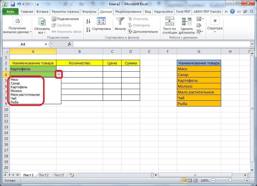
Also in Excel program You can create linked dropdown lists. These are lists where when you select one value from the list, in another column you are asked to select the corresponding parameters. For example, when choosing potatoes in the list of products, you are asked to select kilograms and grams as measurements, and when choosing vegetable oil, liters and milliliters.

First of all, let's prepare a table where the drop-down lists will be located, and separately make lists with the names of products and measures of measurement.

We assign a named range to each of the lists, as we did earlier with regular drop-down lists.

In the first cell, we create a list in exactly the same way as we did earlier, through data verification.

In the second cell we also launch the data verification window, but in the “Source” column we enter the function “=INDIRECT” and the address of the first cell. For example, =INDIRECT($B3).

As you can see, the list has been created.

Now, so that the lower cells acquire the same properties as the previous time, select the upper cells, and while holding down the mouse button, drag them down.

That's it, the table has been created.

We figured out how to make a drop-down list in Excel. In the program you can create both simple drop-down lists and dependent ones. In this case, you can use various creation methods. The choice depends on the specific purpose of the list, the purpose of its creation, the scope of application, etc.

When filling cells with data, it is often necessary to limit the input to a specific list of values. For example, there is a cell where the user must enter the name of the department, indicating where he works. It is logical to first create a list of departments of the organization and allow the user to only select values from this list. This approach will help speed up the input process and reduce the number of typos.

Drop-down list can be created using

In this article we will create Drop-down list using () with data type List.

Drop-down list can be formed in different ways.

A. The simplest drop-down list - entering list items directly into the Source field

Suppose in a cell B 1 need to create drop-down list to enter units of measurement. Select a cell B 1 and call Data verification.

If in the field Source indicate units of measurement separated by semicolons pcs;kg;sq.m;cub.m, then the choice will be limited to these four values.

Now let's see what happened. Select a cell B 1 . When you select a cell, a square arrow button appears to the right of the cell to select items from drop down list.

Flaws this approach: list items are easy to lose (for example, by deleting a row or column containing a cell B 1 ); It is not convenient to enter a large number of elements. The approach is suitable for small (3-5 values) immutable lists.
Advantage: Create a list quickly.

B. Entering list items into a range (on the same sheet as the drop-down list)

Items for a dropdown list can be placed in a range of EXCEL sheet and then into the field Source tool to specify a link to this range.

Suppose the elements of the list pcs;kg;sq.m;cub.m entered into range cells A 1: A 4 , then the field Source will contain =sheet1!$A$1:$A$4

Advantage: clarity of the list of elements and ease of modification. The approach is suitable for lists that change rarely.
Flaws: If new elements are added, you have to manually change the range reference. True, a wider range can be immediately identified as a source, for example, A 1: A 100 . But then the drop-down list may contain empty lines (if, for example, some of the elements were deleted or the list was just created). To make empty lines disappear, you need to save the file.

Second disadvantage: the source range must be located on the same sheet as drop-down list, because rules cannot use links to other sheets or workbooks (this is true for EXCEL 2007 and earlier).

Let's get rid of the second drawback first - we'll post a list of elements drop down list on another sheet.

B. Entering list items into a range (on any worksheet)

Entering list items into a range of cells in another workbook

If you need to move a range with drop-down list items to another workbook (for example, to a workbook Source.xlsx), then you need to do the following:

in the book Source.xlsx create the necessary list of elements;
in the book Source.xlsx assign to the range of cells containing the list of elements, for example ListExt;
open the workbook in which you intend to place the cells with the drop-down list;
select the desired range of cells, call the tool , in field Source indicate = INDIRECT("[Source.xlsx]sheet1!ListExt");

When working with a list of elements located in another workbook, the file Source.xlsx must be open and located in the same folder, otherwise you must specify full path to the file. In general, it is better to avoid references to other sheets or use Personal macro book Personal.xlsx or Add-ons.

If you don't want to assign a name to the range in the file Source.xlsx, then the formula needs to be changed to = INDIRECT("[Source.xlsx]sheet1!$A$1:$A$4")

ADVICE:
If there are many cells with rules on the sheet Data checks, then you can use the tool ( Home/ Find and Select/ Selecting a group of cells). Option Data checking This tool allows you to select cells that are subject to data validation (specified using the command Data/Working with Data/Validating Data). When selecting a switch Everyone all such cells will be selected. When selecting the option These same Only those cells are highlighted that have the same data validation rules as the active cell.

Note:
If drop-down list contains more than 25-30 values, then working with it becomes inconvenient. Drop-down list displays only 8 elements at a time, and to see the rest, you need to use the scroll bar, which is not always convenient.

EXCEL does not provide font size adjustment Dropdown list. With a large number of elements, it makes sense to list elements and use additional classification of elements (i.e., split one drop-down list into 2 or more).

For example, to effectively work with an employee list of more than 300 employees, it should first be sorted alphabetically. Then create drop-down list containing letters of the alphabet. Second drop-down list should contain only those surnames that begin with the letter selected in the first list. To solve such a problem, the or structure can be used.

Good afternoon, dear reader!

In this article, I would like to talk about what a drop-down list in a cell is, how to make it, and, accordingly, what is it for?

This is a list of fixed values that are only available from a specified range of values. This means that the cell you specify can only contain data that corresponds to the values of the specified range; data that does not correspond will not be entered. In a cell, you can select the values that a fixed list in the cell offers.

Well, let's look at creating drop-down lists and why it is needed:

I personally use the dropdown list all the time for all 3 reasons. And it greatly simplifies my work with data; I deliberately reduce the possibility of entering primary data to 0%.

Well, here are 2 questions, what and why, I told you, but we’ll talk about how to do this below.

And we will create a drop-down list in a cell in several stages:

1. Determine the range of cells in which we will create a fixed list.

2. Select the range we need and select the item in the menu “Data” - “Data check”, in the context window that appears, select the item from the specified selection "List".

3. In the line unlocked below, indicate the range of data that should be in our drop-down list. Click "OK" and the job is done.

In older versions of Excel, there is no way to create a drop-down list in a cell using data from other sheets, so it makes sense to create lists in the same sheet and hide them. Also, if necessary, you can create a vertical list - a horizontal one using the feature.

And that's all for me! I really hope that all of the above is clear to you. I would be very grateful for your comments, as this is an indicator of readability and inspires me to write new articles! Share what you read with your friends and like it!

The progress of mankind is based on the desire of every person to live beyond his means
Samuel Butler, philosopher

A drop-down list refers to the content of several values in one cell. When the user clicks on the arrow on the right, a specific list appears. You can choose a specific one.

A very convenient Excel tool for checking entered data. The capabilities of drop-down lists allow you to increase the comfort of working with data: data substitution, display of data from another sheet or file, the presence of a search function and dependencies.

Creating a Dropdown List

Path: Data menu - Data Validation tool - Options tab. Data type – “List”.

You can enter the values from which the drop-down list will be composed in different ways:

Any of the options will give the same result.

Dropdown list in Excel with data substitution

Need to make a dropdown list with values from dynamic range. If changes are made to the existing range (data is added or removed), they are automatically reflected in the drop-down list.

Let's test it. Here is our table with the list on one sheet:

Let’s add a new value “Christmas tree” to the table.

Now let’s remove the “birch” value.

The “smart table”, which easily “expands” and changes, helped us realize our plans.

Now let's make it possible to enter new values directly into the cell with this list. And the data was automatically added to the range.

When we enter a new name into an empty cell of the drop-down list, a message will appear: “Add the entered name baobab to the drop-down list?”

Click “Yes” and add another line with the value “baobab”.

Dropdown list in Excel with data from another sheet/file

When the values for the dropdown list are located on another sheet or in another workbook, standard way does not work. You can solve the problem using the INDIRECT function: it will generate the correct link to external source information.

We make active the cell where we want to place the drop-down list.
Open data verification options. In the “Source” field, enter the formula: =INDIRECT(“[List1.xlsx]Sheet1!$A$1:$A$9”).

The name of the file from which the information for the list is taken is enclosed in square brackets. This file must be open. If the book with the required values is located in another folder, you need to specify the full path.

How to make dependent dropdown lists

Let's take three named ranges:

This is a must. The above describes how to make a regular list a named range (using the “Name Manager”). Remember that the name cannot contain spaces or punctuation marks.

Let's create the first drop-down list, which will include the names of the ranges.

When you have placed the cursor in the “Source” field, go to the sheet and select the required cells one by one.

Now let's create a second dropdown list. It should reflect those words that correspond to the name selected in the first list. If “Trees”, then “hornbeam”, “oak”, etc. Enter in the “Source” field a function of the form =INDIRECT(E3). E3 – cell with the name of the first range.

Selecting multiple values from an Excel dropdown list

It happens when you need to select several items from a drop-down list at once. Let's consider ways to implement the task.

We create standard list using the Data Validation tool. Add to source sheet ready macro. How to do this is described above. With its help, the selected values will be added to the right of the drop-down list.
To make the selected values appear below, we insert another handler code.
To display the selected values in one cell, separated by any punctuation mark, use the following module.

Private Sub Worksheet_Change(ByVal Target As Range)
On Error Resume Next
If Not Intersect(Target, Range("C2:C5")) Is Nothing And Target.Cells.Count = 1 Then
Application.EnableEvents = False
newVal = Target
Application.Undo
oldval = Target
If Len(oldval)<>0 And oldval<>newValThen
Target = Target & "," & newVal
Else
Target = newVal
End If
If Len(newVal) = 0 Then Target.ClearContents
Application.EnableEvents = True
End If
End Sub

Don’t forget to change the ranges to “your own”. We create lists in the classic way. And macros will do the rest of the work.

Dropdown list with search

When you enter the first letters on the keyboard, matching elements are highlighted. And these are not all the pleasant aspects of this tool. Here you can customize the visual presentation of information and specify two columns as a source at once.

Popular in the category: