Ms sql server writing queries. Executing SQL queries in Management Studio. Adding an Average calculated field
Table expressions are called subqueries that are used where the presence of a table is expected. There are two types of table expressions:
derived tables;
generalized table expressions.
These two forms of table expressions are discussed in the following subsections.
Derived tables
Derived table is a table expression included in the FROM clause of a query. Derived tables can be used in cases where using column aliases is not possible because the SQL translator processes another statement before the alias is known. The example below shows an attempt to use a column alias in a situation where another clause is being processed before the alias is known:
USE SampleDb; SELECT MONTH(EnterDate) as enter_month FROM Works_on GROUP BY enter_month;
Trying to run this query will produce the following error message:
Msg 207, Level 16, State 1, Line 5 Invalid column name "enter_month". (Message 207: Level 16, State 1, Line 5 Invalid column name enter_month)
The reason for the error is that the GROUP BY clause is processed before the corresponding list of the SELECT statement is processed, and the enter_month column alias is unknown when the group is processed.
This problem can be solved by using a derived table that contains the preceding query (without the GROUP BY clause) because the FROM clause is executed before the GROUP BY clause:
USE SampleDb; SELECT enter_month FROM (SELECT MONTH(EnterDate) as enter_month FROM Works_on) AS m GROUP BY enter_month;
The result of this query will be like this:
Typically, a table expression can be placed anywhere in a SELECT statement where a table name might appear. (The result of a table expression is always a table or, in special cases, an expression.) The example below shows the use of a table expression in the select list of a SELECT statement:
The result of this query:

Generic table expressions
Common Table Expression (OTB) is a named table expression supported by the Transact-SQL language. Common table expressions are used in the following two types of queries:
non-recursive;
recursive.
These two types of requests are discussed in the following sections.
OTB and non-recursive queries
The non-recursive form of OTB can be used as an alternative to derived tables and views. Typically OTB is determined by WITH clauses and an additional query that references the name used in the WITH clause. In Transact-SQL, the meaning of the WITH keyword is ambiguous. To avoid ambiguity, the statement preceding the WITH statement should be terminated with a semicolon.
USE AdventureWorks2012; SELECT SalesOrderID FROM Sales.SalesOrderHeader WHERE TotalDue > (SELECT AVG(TotalDue) FROM Sales.SalesOrderHeader WHERE YEAR(OrderDate) = "2005") AND Freight > (SELECT AVG(TotalDue) FROM Sales.SalesOrderHeader WHERE YEAR(OrderDate) = "2005 ")/2.5;
The query in this example selects orders whose total taxes (TotalDue) are greater than the average of all taxes and whose freight charges (Freight) are greater than 40% of the average taxes. The main property of this query is its length, since the subquery needs to be written twice. One of possible ways to reduce the size of the query construct would be to create a view containing a subquery. But this solution is a bit complicated because it requires creating a view and then deleting it after the query has finished executing. A better approach would be to create an OTB. The example below shows the use of non-recursive OTB, which shortens the query definition above:
USE AdventureWorks2012; WITH price_calc(year_2005) AS (SELECT AVG(TotalDue) FROM Sales.SalesOrderHeader WHERE YEAR(OrderDate) = "2005") SELECT SalesOrderID FROM Sales.SalesOrderHeader WHERE TotalDue > (SELECT year_2005 FROM price_calc) AND Freight > (SELECT year_2005 FROM price_cal c) /2.5;
The WITH clause syntax in non-recursive queries is as follows:
The cte_name parameter represents the OTB name that defines the resulting table, and the column_list parameter represents the list of columns of the table expression. (In the example above, the OTB is called price_calc and has one column, year_2005.) The inner_query parameter represents a SELECT statement that specifies the result set of the corresponding table expression. The defined table expression can then be used in the outer_query. (The outer query in the example above uses OTB price_calc and its year_2005 column to simplify the doubly nested query.)
OTB and recursive queries
This section presents material of increased complexity. Therefore, when reading it for the first time, it is recommended to skip it and return to it later. OTBs can be used to implement recursions because OTBs can contain references to themselves. The basic OTB syntax for a recursive query looks like this:
The cte_name and column_list parameters have the same meaning as in OTB for non-recursive queries. The body of a WITH clause consists of two queries combined by the operator UNION ALL. The first query is called only once, and it begins to accumulate the result of the recursion. The first operand of the UNION ALL operator does not reference OTB. This query is called a reference query or source.
The second query contains a reference to the OTB and represents its recursive part. Because of this, it is called a recursive member. In the first call to the recursive part, the OTB reference represents the result of the reference query. The recursive member uses the result of the first query call. After this, the system calls the recursive part again. A call to a recursive member stops when a previous call to it returns an empty result set.
The UNION ALL operator joins the currently accumulated rows, as well as additional rows added by the current call to the recursive member. (The presence of the UNION ALL operator means that duplicate rows will not be removed from the result.)
Finally, the outer_query parameter specifies the outer query that OTB uses to retrieve all calls to the join of both members.
To demonstrate the recursive form of OTB, we use the Airplane table defined and populated with the code shown in the example below:
USE SampleDb; CREATE TABLE Airplane(ContainingAssembly VARCHAR(10), ContainedAssembly VARCHAR(10), QuantityContained INT, UnitCost DECIMAL(6,2)); INSERT INTO Airplane VALUES ("Airplane", "Fuselage", 1, 10); INSERT INTO Airplane VALUES ("Airplane", "Wings", 1, 11); INSERT INTO Airplane VALUES ("Airplane", "Tail", 1, 12); INSERT INTO Airplane VALUES ("Fuselage", "Salon", 1, 13); INSERT INTO Airplane VALUES ("Fuselage", "Cockpit", 1, 14); INSERT INTO Airplane VALUES ("Fuselage", "Nose",1, 15); INSERT INTO Airplane VALUES ("Cabin", NULL, 1,13); INSERT INTO Airplane VALUES ("Cockpit", NULL, 1, 14); INSERT INTO Airplane VALUES ("Nose", NULL, 1, 15); INSERT INTO Airplane VALUES ("Wings", NULL,2, 11); INSERT INTO Airplane VALUES ("Tail", NULL, 1, 12);
The Airplane table has four columns. The ContainingAssembly column identifies the assembly, and the ContainedAssembly column identifies the parts (one by one) that make up the corresponding assembly. The figure below shows a graphic illustration of a possible type of aircraft and its component parts:

The Airplane table consists of the following 11 rows:

The following example uses the WITH clause to define a query that calculates the total cost of each build:
USE SampleDb; WITH list_of_parts(assembly1, quantity, cost) AS (SELECT ContainingAssembly, QuantityContained, UnitCost FROM Airplane WHERE ContainedAssembly IS NULL UNION ALL SELECT a.ContainingAssembly, a.QuantityContained, CAST(l.quantity * l.cost AS DECIMAL(6,2) ) FROM list_of_parts l, Airplane a WHERE l.assembly1 = a.ContainedAssembly) SELECT assembly1 "Part", quantity "Quantity", cost "Price" FROM list_of_parts;
The WITH clause defines an OTB list named list_of_parts, consisting of three columns: assembly1, quantity, and cost. The first SELECT statement in the example is called only once to store the results of the first step of the recursion process. The SELECT statement on the last line of the example displays the following result.
SQL or Structured Query Language is a language used to manage data in a relational database system (RDBMS). This article will cover commonly used SQL commands, which every programmer should be familiar with. This material is ideal for those who want to brush up on their knowledge of SQL before a job interview. To do this, look at the examples given in the article and remember that you studied databases in pairs.
Note that some database systems require a semicolon at the end of each statement. The semicolon is standard pointer at the end of every statement in SQL. The examples use MySQL, so a semicolon is required.
Setting up a database for examples
Create a database to demonstrate how teams work. To work, you will need to download two files: DLL.sql and InsertStatements.sql. After that, open a terminal and log into the MySQL console using the following command (the article assumes that MySQL is already installed on the system):
Mysql -u root -p
Then enter your password.
Run the following command. Let's call the database “university”:
CREATE DATABASE university; USE university; SOURCE You may need to create restrictions on certain columns in a table. When creating a table, you can set the following restrictions: You can specify more than one primary key. In this case, you will get a composite primary key. Create a table "instructor": CREATE TABLE instructor (ID CHAR(5), name VARCHAR(20) NOT NULL, dept_name VARCHAR(20), salary NUMERIC(8,2), PRIMARY KEY (ID), FOREIGN KEY (dept_name) REFERENCES department(dept_name)); You can view various information (value type, key or not) about table columns with the following command: DESCRIBE When you add data to each column in a table, you do not need to specify column names. INSERT INTO SELECT is used to retrieve data from a specific table: SELECT The following command can display all the data from the table: SELECT * FROM Table columns may contain duplicate data. Use SELECT DISTINCT to retrieve only non-duplicate data. SELECT DISTINCT You can use the WHERE keyword in SELECT to specify conditions in a query: SELECT The following conditions can be specified in the request: Try the following commands. Pay attention to the conditions specified in WHERE: SELECT * FROM course WHERE dept_name=’Comp. Sci.'; SELECT * FROM course WHERE credits>3; SELECT * FROM course WHERE dept_name="Comp. Sci." AND credits>3; The GROUP BY operator is often used with aggregate functions such as COUNT, MAX, MIN, SUM and AVG to group output values. SELECT Let's display the number of courses for each faculty: SELECT COUNT(course_id), dept_name FROM course GROUP BY dept_name; The HAVING keyword was added to SQL because WHERE cannot be used with aggregate functions. SELECT Let's display a list of faculties that have more than one course: SELECT COUNT(course_id), dept_name FROM course GROUP BY dept_name HAVING COUNT(course_id)>1; ORDER BY is used to sort query results in descending or ascending order. ORDER BY will sort in ascending order unless ASC or DESC is specified. SELECT Let's display a list of courses in ascending and descending order of credits: SELECT * FROM course ORDER BY credits; SELECT * FROM course ORDER BY credits DESC; BETWEEN is used to select data values from a specific range. Numeric and text values, as well as dates. SELECT Let's display a list of instructors whose salary is more than 50,000, but less than 100,000: SELECT * FROM instructor WHERE salary BETWEEN 50000 AND 100000; The LIKE operator is used in WHERE to specify a search pattern for a similar value. There are two free operators that are used in LIKE: Let's display a list of courses whose names contain "to" and a list of courses whose names begin with "CS-": SELECT * FROM course WHERE title LIKE ‘%to%’; SELECT * FROM course WHERE course_id LIKE "CS-___"; Using IN you can specify multiple values for the WHERE clause: SELECT Let's display a list of students from Comp majors. Sci., Physics and Elec. Eng.: SELECT * FROM student WHERE dept_name IN ('Comp. Sci.', 'Physics', 'Elec. Eng.'); JOIN is used to link two or more tables using common attributes within them. The image below shows various ways joins in SQL. Note the difference between a left outer join and a right outer join: SELECT We will display a list of all courses and relevant information about the faculties: SELECT * FROM course JOIN department ON course.dept_name=department.dept_name; We will display a list of all required courses and details about them: SELECT prereq.course_id, title, dept_name, credits, prereq_id FROM prereq LEFT OUTER JOIN course ON prereq.course_id=course.course_id; We will display a list of all courses, regardless of whether they are required or not: SELECT course.course_id, title, dept_name, credits, prereq_id FROM prereq RIGHT OUTER JOIN course ON prereq.course_id=course.course_id; View is a virtual SQL table created as a result of executing an expression. It contains rows and columns and is very similar to a regular SQL table. View always shows the latest information from the database. Let's create a view consisting of courses with 3 credits: These functions are used to obtain an aggregate result related to the data in question. The following are commonly used aggregate functions: Nested subqueries are SQL queries that include SELECT , FROM , and WHERE clauses nested within another query. Let's find courses that were taught in the fall of 2009 and spring of 2010: SELECT DISTINCT course_id FROM section WHERE semester = 'Fall' AND year= 2009 AND course_id IN (SELECT course_id FROM section WHERE semester = 'Spring' AND year= 2010); SQL - Structured Query Language. Description
bigint (int 8) bigint (int 8) binary(n) binary(n) or image character national character or ntext character varying(synonym char varying varchar) national character varying or ntext Datetime datetime decimal aka numeric double precision double precision integer (int 4) (synonym: int) integer (int 4) national character(synonym: national character, nchar) national character Numeric(synonyms: decimal, dec) national character varying(synonyms: national char varying, nvarchar) National character varying Smalldatetime datetime smallint (int 2) smallint (int 2) Smallmoney sql_variant No longer supported Ntext Timestamp Not supported tinyint (int 1) tinyint (int 1) Uniqueidentifier uniqueidentifier varbinary(n) varbinary(n) or image smalldatetime datetime smallint (int 2) smallint (int 2) smallmoney sql_variant Not supported timestamp Not supported tinyint (int 1) tinyint (int 1) uniqueidentifier uniqueidentifier varbinary(n) varbinary(n) or image Data Type Table in SQL Server 2000 Request is a command you give to your database program. Queries are part of the DML language. All SQL queries consist of a single command. The structure of this command is deceptively simple because you must extend it to perform highly complex evaluations and data manipulations. SELECT“Select” is the most frequently used command; it is used to select data from the table. SELECT id, user_name, city, birth_day FROM users_base; Such a query will display from the users_base table all the values of the columns specified separated by commas after SELECT commands. Also, you can display all columns with one character, * i.e. SELECT * FROM users_base ; - such a query will display all data from the table. SELECT (Column names separated by commas that need to be displayed in the query) FROM (table name in the database) Values can be placed and removed from fields using three DML (Data Manipulation Language) commands: INSERT INTO users_base (user_name, city, birth_day) VALUES ('Alexander', 'Rostov', '06/20/1991'); UPDATE users_base SET user_name = 'Alexey'; The UPDATE command updates values in a table. First comes the UPDATE command itself, then the table name, after the SET command (set), then the column name and its value in quotes (quotes are placed if the value is in string format, if it is a numeric value and the column is not tied to the data type vchar or any other string types, the quotes have no meaning.) DELETE FROM users_base WHERE user_name = 'Vasily'; The DELETE command deletes the entire row and identifies the row using the WHERE criterion. In this case, this query would delete all rows in which the user_name column value was Vasily. We'll talk about the WHERE criterion and others a little later. WHERE clause is a clause of the SELECT command and other DML commands that allows you to set predicates whose condition can be either true or false for any row in the table. The command retrieves only those rows from the table for which this statement is true. ORDER BY - condition for sorting the selected rows. Has 2 criteria ASC and DESC. ASC (sorting from A to Z or from 0 to 9) DESC (opposite of ASC). This condition can also be used in conjunction with the WHERE clause. DISTINCT is an argument that provides you with a way to eliminate double values from your SELECT clause. Those. if you have duplicate values in a column, let’s say user_name, then DISTINCT will show you only one value, for example, you have 2 people named Alexey in your database, then a query using the DISTINCT function will show you only 1 value that is encountered first... AND - takes two Boolean (in the form A AND B) as arguments and evaluates them against the truth whether they are both true. OR - takes two Boolean (in the form A OR B) as arguments and evaluates whether one of them is correct. SELECT * FROM users_base WHERE city = 'Rostov' OR user_name = 'Alexander';- will display all values from the table where the name of the city of Rostov or the username Alexander appears in the line. NOT - takes a single Boolean (in the form NOT A) as arguments and changes its value from false to true or true to false. IN - defines a set of values in which a given value may or may not be included. Between is similar to the IN operator. Unlike defining by numbers from a set, as IN does, BETWEEN defines a range whose values must decrease to make the predicate true. COUNT - Produces the row numbers or non-NULL values of the fields that the query selected. SUM - produces the arithmetic sum of all selected values for a given field. AVG - averages all selected values of this field. MAX - produces the largest of all selected values for this field. MIN - produces the smallest of all selected values for this field. CREATE TABLE users_base (id integer, user_name text, city text, birth_day datetime);- executing such a command will lead to the creation of the table for which I gave examples... Everything is simple here, we write the CREATE TABLE command, followed by the name of the table that we want to create, then in parentheses, separated by commas, the names of the columns and their data type. This is the standard way to create a table in SQL. Now I will give an example of creating tables in SQL Server 2005: SET ANSI_NULLS ON If you have any questions on this topic, please write to me Develop an application that demonstrates basic operations on data in a database such as MS SQL Server, namely: The Education.dbo database is taken as a basis, the creation process of which is described in detail Figure 1 shows the structure of the Education.dbo database. As can be seen from the figure, the database is called: Here “sasha-pc” is the computer identifier on the network, “sqlexpress” is the name of the database server, “Education.dbo” is the name of the database. Rice. 1. Education.dbo database The database contains two tables: Student and Session. The structure of the tables is as follows. Student table. Session table. Create a new project of type Windows Forms Application. An example of creating a new project is described in detail To display data from database tables, you can use different ways. One of them is the creation of views, which are generated using MS Visual Studio. In our case, the table data will be displayed on the form in a control of the DataGridView type. After creating views, it is very convenient to associate them with DataGridView elements. To create a view, you need to call the “Add New View” command from the context menu, which is called by right-clicking on the “Views” element of the Education.dbo database (Figure 2). Rice. 2. Calling the command to add a new view As a result, the “Add Table" window will open (Figure 3). In the window you need to select the tables that are added to the view. Rice. 3. Selecting the tables on which the new view will be based In our case, select the Student table and confirm your choice by clicking on the Add button. The next step is to close the window by selecting the Close button. After completing the steps, a window will be generated in which you need to select the fields that should be displayed in the view (on the form). Select all fields (Figure 4). When you select fields, the fields of the Student table are displayed at the top of the work area. Using the mouse, you can select the desired fields for presentation. Accordingly, the middle area of the window displays the names of the selected fields, the table in which they exist (see Fig. 4), the ability to sort, filter, etc. The bottom of the area displays the corresponding SQL query text that is used to create the view. Rice. 4. Selecting Student table fields to display in the view After choosing a team A window will open in which you need to specify the name of the view. Set the name “View Student” (Figure 5). Rice. 5. Specifying a name for the view After completing the steps, the presentation window will look like shown in Figure 6. Rice. 6. View Student representation in the database You can now host a DataGridView control and associate it with a view. Before placing the DataGridView control, you need to go into form design mode "Form1.cs". The DataGridView element is a table that can display data. This control is located in the ToolBox panel. First, we slightly adjust the size of the form, and then place the DataGridView control on it (Figure 7). This will create an object instance named dataGridView1 by default. Rice. 7. DataGridView control and data source selection window After placing the DataGridView control on the form, in the upper right corner you can choose to configure the data source. Accordingly, the “DataGridView Tasks" window will open. In this window you need to select the “Choose Data Source” pop-up menu. In the menu that opens, select the “Add Project Data Source...” command (Fig. 7). After this, a wizard window opens, in which the data source is sequentially selected. Figure 8 shows the " Data Source Configuration Wizard“, in which the type of data source is selected. In our case, we install “Database“. Rice. 8. Selecting a data source type In the next window (Figure 9) the data source model is selected. You need to select DataSet. Rice. 9. Selecting a data source model In the window shown in Figure 10, you need to specify the data connection that you want to use to connect to the database. In our case, we need to select the database " sasha-pc\sqlexpress\Education.dbo«.
Rice. 10. Selecting a data connection The next window (Figure 11) suggests saving the Connection String to the application configuration file. We leave everything as is and move on to the next window. Rice. 11. Proposal for saving the database connection string Connection String in the application configuration file After creating a database connection, a variety of database objects are displayed (Figure 12). In our case, we need to select the “View Student” view and all the fields from it. The checked fields will be displayed in the DataGridView type component. Rice. 12. Selecting the Database Objects to Display in the DataGridView After selecting the Finish button, the selected objects (View Student view) of the Education.dbo database will be displayed (Figure 13). Rice. 13. DataGridView control with selected View Student fields In a similar way, you can configure views that contain any fields from any database table. Also, fields from different tables can be displayed in one view. If you run the application, you will receive data from the View Student view, which corresponds to the Student table in the database (Figure 14). As you can see from Figure 14, the data in the dataGridView1 table is displayed normally, but the design can be adjusted. A control of the DataGridView type allows you to adjust the appearance of the fields that are displayed. To call commands for editing fields, just call the context menu by right-clicking on the dataGridView1 control. The menu has various useful commands, which allow you to control the appearance and operation of the DataGridView: In our case, you need to select the “Edit Columns...” command (Figure 15). Rice. 15. Command “Edit Columns...” from the context menu As a result, the “Edit Columns” window will open, in which you can customize the appearance of the presentation fields to your liking (Figure 16). In the window in Figure 16, for any field you can configure the name, alignment, width, ability to edit data, etc. In order to make changes to the database, you need to get a connection string to the database Connection String . There are different ways to get the database connection string. One of them is based on reading this line in the Properties window of the Education.dbo database (Fig. 17). To save the string in the program, an internal variable of the type string. Using the clipboard, copy the Connection String into the described string variable. In the text of the file “Form1.cs" at the beginning of the description of the Form1 class, you need to describe the variable: At the moment the text of the Form1 class is as follows: In order to be able to process the data of the current record, you need to create a new form. The process of creating a new form in MS Visual Studio - C# is described in detail. Adding a new form is done with the command: In the “New Item” window that opens, you need to select the “Windows Form“ element. Leave the new form file name as default “Form2.cs”. Figure 18 shows a view of the new form. We place the following types of controls on the form: You need to configure the following properties of the controls: We also configure the visibility of TextBox controls. To do this, in all controls textBox1, textBox2, textBox3, textBox4, the property value Modifiers = “public”. For further work, you need to use the mouse to switch to the main form Form1. Add three buttons to the main form of the Form1 application (Button). Three object variables will be automatically created with the names button1, button2, button3. In each of these buttons we make the following settings (Properties window): As a result of the changes made, the main form will look like shown in Figure 19. The click event handler on the “Insert...” button looks like this: Form2 is called first. After receiving the “OK” result (pressing the corresponding button), in Form2 the filled fields in elements of the TextBox type are included in the SQL query string. The SQL query for adding a new row looks like: where value1 corresponds to the grade book number; value2 – student’s last name; value3 – group in which the student studies; value4 – year of entry. The Connection String database connection string is described in the conn_string variable (see paragraph 5). The SqlConnection class object connects the application to data sources. In addition, the Connection class handles user authentication, networking, database identification, connection buffering, and transaction processing. The SQL command that adds a record to a table is encapsulated in the SqlCommand class. The constructor of the SqlCommand class takes two parameters: a SQL query string (cmd_text variable) and an object of the SqlConnection class. The ExecuteNonQuery() method is implemented in the IDBCommand interface. The method implements SQL commands that do not return data. Such commands include INSERT, DELETE, UPDATE commands, as well as stored procedures that do not return data. The ExecuteNonQuery() method returns the number of records involved. The click event handler on the “Edit...” button looks like this: This handler executes an UPDATE SQL command that changes the current value of the active record. The click event handler on the “Delete” button looks like this: This handler executes the SQL command DELETE to delete a record. SQL Server Management Studio provides a complete tool for creating all types of queries. With its help you can create, save, load and edit queries. In addition, you can work on queries without connecting to any server. This tool also provides the ability to develop queries for different projects. You can work with queries using either the Query Editor or the Solution Explorer. This article covers both of these tools. In addition to these two components of SQL Server Management Studio, we'll look at debugging SQL code using the built-in debugger. To open the Query Editor panel Query Editor, on the SQL Server Management Studio toolbar, click the New Query button. This panel can be expanded to display buttons for creating all possible queries, not just Database Engine queries. By default it is created new request Database Engine component, but by clicking the corresponding button on the toolbar, you can also create MDX, XMLA, etc. queries. The status bar at the bottom of the Query Editor panel indicates the status of the editor's connection to the server. If you do not connect to the server automatically, when you launch the Query Editor, a Connect to Server dialog box appears, allowing you to select the server to connect to and the authentication mode. Editing queries offline provides more flexibility than when connected to a server. To edit queries, it is not necessary to connect to the server, and the query editor window can be disconnected from one server (using the menu command Query --> Connection --> Disconnect) and connected to another without opening another editor window. To select offline editing mode, use the Connect to Server dialog that opens when you launch the editor. specific type requests, simply click the Cancel button. You can use the Query Editor to perform the following tasks: creating and executing Transact-SQL statements; saving created Transact-SQL language statements to a file; creating and analyzing execution plans for common queries; graphically illustrating the execution plan of the selected query. The query editor contains a built-in text editor and a toolbar with a set of buttons for different actions. The main query editor window is divided horizontally into a query panel (at the top) and a results panel (at the bottom). Transact-SQL statements (that is, queries) to be executed are entered in the top pane, and the results of the system's processing of those queries are displayed in the bottom pane. The figure below shows an example of entering a query into the query editor and the results of executing that query: The first USE request statement specifies to use the SampleDb database as the current database. The second statement, SELECT, retrieves all rows from the Employee table. To run this query and display the results, on the Query Editor toolbar, click the Execute button or press F5. You can open several Query Editor windows, i.e. make multiple connections to one or more instances of the Database Engine. A new connection is created by clicking the New Query button on the SQL Server Management Studio toolbar. The status bar at the bottom of the Query Editor window displays the following information related to the execution of query statements: the status of the current operation (for example, "Request completed successfully"); database server name; current user name and server process ID; current database name; time spent executing the last request; number of lines found. One of the main advantages of SQL Server Management Studio is its ease of use, which also applies to the Query Editor. The Query Editor provides many features to make coding Transact-SQL statements easier. In particular, it uses syntax highlighting to improve the readability of Transact-SQL statements. All reserved words are shown in blue, variables are shown in black, strings are shown in red, and comments are shown in green. In addition, the query editor is equipped with context-sensitive help called Dynamic Help, through which you can obtain information about a specific instruction. If you don't know the syntax of an instruction, select it in the editor, and then press the F1 key. You can also highlight the parameters of various Transact-SQL statements to get help about them from Books Online. SQL Management Studio supports SQL Intellisense, which is a type of auto-completion tool. In other words, this module suggests the most likely completion of partially entered Transact-SQL statement elements. The object explorer can also help you edit queries. For example, if you want to know how to create a CREATE TABLE statement for the Employee table, right-click the table in Object Explorer and the resulting context menu select Script Table As --> CREATE to --> New Query Editor Window. The Query Editor window containing the CREATE TABLE statement created in this way is shown in the figure below. This feature also applies to other objects, such as stored procedures and functions. The Object Browser is very useful for graphically displaying the execution plan of a particular query. The query execution plan is the execution option selected by the query optimizer among several possible options fulfilling a specific request. Enter the required query in the top panel of the editor, select a sequence of commands from the Query --> Display Estimated Execution Plan menu, and the execution plan for this query will be shown in the bottom panel of the editor window. Query editing in SQL Server Management Studio is based on the solutions method. If you create an empty query using the New Query button, it will be based on an empty solution. You can see this by running a sequence of commands from the View --> Solution Explorer menu immediately after opening an empty query. The decision may be related to none, one, or several projects. An empty solution, not associated with any project. To associate a project with a solution, close the empty solution, Solution Explorer, and Query Editor, and create a new project by running File --> New --> Project. In the New Project window that opens, select the SQL Server Scripts option in the middle pane. A project is a way of organizing files in a specific location. You can assign a name to the project and choose a location for its location on disk. When you create a new project, a new solution is automatically launched. The project can be added to existing solution using Solution Explorer. For each project created, Solution Explorer displays the Connections, Queries, and Miscellaneous folders. To open a new Query Editor window for a given project, right-click its Queries folder and select New Query from the context menu. SQL Server, starting with SQL Server 2008, has a built-in code debugger. To begin a debugging session, select Debug --> Start Debugging from the SQL Server Management Studio main menu. We will look at how the debugger works using an example using a batch of commands. A batch is a logical sequence of SQL statements and procedural extensions that is sent to the Database Engine to execute all of the statements it contains. The figure below shows a package that counts the number of employees working on project p1. If this number is 4 or more, then a corresponding message is displayed. Otherwise, the first and last names of the employees are displayed. To stop the execution of a package at a specific instruction, you can set breakpoints, as shown in the figure. To do this, click to the left of the line you want to stop on. When debugging begins, execution stops at the first line of code, which is marked with a yellow arrow. To continue execution and debugging, select the Debug --> Continue menu command. The batch instructions will continue to execute until the first breakpoint, and the yellow arrow will stop at that point. Information related to the debugging process is displayed in two panels at the bottom of the Query Editor window. Information about different types Debugging information is grouped in these panels on several tabs. The left pane contains the Autos tab, Locals tab, and up to five Watch tabs. The right pane contains the Call Stack, Threads, Breakpoints, Command Window, Immediate Window, and Output tabs. The Locals tab displays variable values, the Call Stack tab displays call stack values, and the Breakpoints tab displays breakpoint information. To end the debugging process, execute a sequence of commands from the main menu Debug --> Stop Debugging or click the blue button on the debugger toolbar. SQL Server 2012 adds several new features to the built-in debugger in SQL Server Management Studio. Now you can perform a number of the following operations in it: Specify a breakpoint condition. Breakpoint condition is an SQL expression whose evaluated value determines whether code execution will stop at a given point or not. To specify a breakpoint condition, right-click the red breakpoint icon and select Condition from the context menu. The Breakpoint Condition dialog box opens, allowing you to enter the required Boolean expression. In addition, if you need to stop execution if the expression is true, you should set the Is True switch. If execution needs to be stopped if the expression has changed, then you need to set the When Changed switch. Specify the number of hits at the breakpoint. The hit count is the condition for stopping execution at a given point based on the number of times that breakpoint was hit during execution. When the specified number of passes and any other condition specified for a given breakpoint is reached, the debugger performs the specified action. The execution abort condition based on the number of hits can be one of the following: unconditional (default action) (Break always); if the number of hits is equal to the specified value (Break when the his count equals a specified value); if the number of hits is a multiple of a specified value (Break when the hit count equals a multiple of a specified value); Break when the his count is greater or equal to a specified value. To set the number of hits during debugging, right-click the required breakpoint icon on the Breakpoints tab, select Hit Count from the context menu, then select one of the conditions in the Breakpoint Hit Count dialog box that opens from the previous list. For options that require a value, enter it in the text box to the right of the conditions drop-down list. To save the specified conditions, click OK. Specify a breakpoint filter. A breakpoint filter limits breakpoint operation to only specified computers, processes, or threads. To set a breakpoint filter, right-click the breakpoint you want and select Filter from the context menu. Then, in the Breakpoint Filters dialog box that opens, specify the resources that you want to restrict execution of this breakpoint to. To save the specified conditions, click OK. Specify an action at a breakpoint. The When Hit condition specifies the action to take when batch execution hits a given breakpoint. By default, when both the hit count condition and the stopping condition are satisfied, then execution is aborted. Alternatively, a pre-specified message can be displayed. To specify what to do when a breakpoint is hit, right-click the red icon for the breakpoint and select When Hit from the context menu. In the When Breakpoint is Hit dialog box that opens, select the action you want to take. To save the specified conditions, click OK. Use the Quick Watch window. You can view the value of a Transact-SQL expression in the QuickWatch window, and then save the expression in the Watch window. To open the Quick Watch window, select Quick Watch from the Debug menu. The expression in this window can either be selected from the Expression drop-down list or entered into this field. Use the Quick Info tooltip. When you hover your mouse over a code ID, Quick Info ( Brief information) displays its ad in a pop-up window.Commands for working with databases
1. View available databases
SHOW DATABASES; 2. Create a new database
CREATE DATABASE; 3. Selecting a database to use
USE 4. Import SQL commands from a .sql file
SOURCE 5. Delete the database
DROP DATABASE Working with tables
6. View the tables available in the database
SHOW TABLES; 
7. Create a new table
CREATE TABLE Integrity Constraints When Using CREATE TABLE
Example
8. Table information

9. Adding data to the table
INSERT INTO 10. Updating table data
UPDATE 11. Removing all data from the table
DELETE FROM 12. Delete a table
DROP TABLE Commands for creating queries
13. SELECT

14. SELECT DISTINCT

15. WHERE
Example

16. GROUP BY
Example

17. HAVING
Example

18. ORDER BY
Example

19. BETWEEN
Example

20. LIKE
SELECT Example

21. IN
Example

22. JOIN

Example 1

Example 2

Example 3

23. View
Creation
CREATE VIEW Removal
DROP VIEW Example

24. Aggregate functions
25. Nested subqueries
Example

IN this review We will look at the most common types of SQL queries.
The SQL standard is defined ANSI(American National Standards Institute).
SQL is a language aimed specifically at relational databases. SQL partitioning:
DDL(Data Definition Language)
- the so-called Schema Description Language in ANSI, consists of commands that create objects (tables, indexes, views, and so on) in the database.
DML(Data Manipulation Language) is a set of commands that determine what values are represented in tables at any given time.
DCD(Data Management Language) consists of facilities that determine whether to allow a user to perform certain actions or not. They are part of ANSI DDL. Don't forget these names. These are not different languages, but sections of SQL commands grouped by their functions. Data types:
SQL Server - Data Types
(synonym char)
Starting with SQL Server 2005, it is not recommended for use.
WHAT IS A REQUEST?
SELECT command:
Type of query using SELECT:SELECT command structure:
- This is the simplest type of request. There are additional commands for convenient data retrieval (see below “Functions”) DML commands:
INSERT(Insert)
UPDATE(Update, modification),
DELETE(Delete) INSERT command:
The INSERT command comes with the prefix INTO (in to), then in brackets are the names of the columns into which we must insert data, then comes the VALUES command (values) and in brackets the values come in turn (it is necessary to observe the order of the values with the columns , the values must be in the same order as the columns you specified). UPDATE command:
DELETE command:
Criteria, functions, conditions, etc. what helps us in SQL:
Example:
SELECT id, city, birth_day FROM users_base WHERE user_name = ‘Alexey’;- such a query will display only those rows that match the WHERE condition, namely all rows in which the user_name column has the value Alexey.
Example:
SELECT id, city, birth_day FROM users_base ORDER BY user_name ASC; - such a query will display values sorted by the user_name column from A to Z (A-Z; 0-9)
Example:
SELECT id, city, birth_day FROM users_base WHERE user_name = ‘Alexey’ ORDER BY id ASC;
Example:
SELECT DISTINCT user_name FROM users_base;- such a query will show us the values of all records in the user_name column, but they will not be repeated, i.e. if you had an infinite number of repeating values, then they will not be shown...
Example:
SELECT * FROM users_base WHERE city = 'Rostov' AND user_name = 'Alexander';- will display all the values from the table where the name of the city appears in one line (in this case, Rostov and the user name Alexander.
SELECT * FROM users_base WHERE city = 'Rostov' OR NOT user_name = 'Alexander';- will display all values from the table where the name of the city of Rostov appears in one line or the user name is not exactly Alexander.
SELECT * FROM users_base WHERE city IN ('Vladivostok', 'Rostov');- such a query will display all values from the table that contain the names of the specified cities in the city column
SELECT * FROM users_base WHERE id BETWEEN 1 AND 10;- displays all values from the table that will be in the range from 1 to 10 in the id column
SELECT COUNT (*) FROM users_base ;- will display the number of rows in this table.
SELECT COUNT (DISTINCT user_name) FROM users_base ;- will display the number of lines with user names (not repeated)
SELECT SUM (id) FROM users_base ;- will display the sum of the values of all rows of the id column.
SELECT AVG (id) FROM users_base ;- will display the average of all selected values of the id columnCreating tables:
GO
SET QUOTED_IDENTIFIER ON
GO
IF NOT EXISTS (SELECT * FROM sys.objects WHERE object_id = OBJECT_ID(N."") AND type in (N"U"))
BEGIN
CREATE TABLE .(
NOT NULL,
NOT NULL,
NOT NULL,
PRIMARY KEY CLUSTERED
A.S.C.
END
GO
SET ANSI_NULLS ON
GO
SET QUOTED_IDENTIFIER ON
GO
IF NOT EXISTS (SELECT * FROM sys.objects WHERE object_id = OBJECT_ID(N."") AND type in (N"U"))
BEGIN
CREATE TABLE .(
IDENTITY(1,1) NOT NULL,
NULL,
NULL,
PRIMARY KEY CLUSTERED
A.S.C.
)WITH (IGNORE_DUP_KEY = OFF) ON
) ON TEXTIMAGE_ON
END
GO
SET ANSI_NULLS ON
GO
SET QUOTED_IDENTIFIER ON
GO
IF NOT EXISTS (SELECT * FROM sys.objects WHERE object_id = OBJECT_ID(N."") AND type in (N"U"))
BEGIN
CREATE TABLE .(
IDENTITY(1,1) NOT NULL,
NULL,
NULL,
PRIMARY KEY CLUSTERED
A.S.C.
)WITH (IGNORE_DUP_KEY = OFF) ON
) ON
END
Syntax in SQL Server 2005 is another topic, I just wanted to show that I described the basics of SQL programming, you can reach the top by yourself knowing the basics.

Performance
1. Create a new project in MS Visual Studio as Windows Forms Application.
2. Create a new view to display data from the Student table.


3. Place the DataGridView control and configure the connection with the database.


4. Setting the appearance of the DataGridView control.
 Rice. 14. Launching the application for execution
 Rice. 16. Window for setting up the view of fields in the “View Student” view
5. Connection String
 Rice. 17. Defining a Connection String
6. Creation new form to demonstrate data manipulation commands.
 Rice. 18. View of the newly created form
7. Adding buttons for calling commands for manipulating data from the Student table.
 Rice. 19. Main form of the application
8. Programming a click event on the “Insert...” button.
9. Programming a click event on the “Edit...” button.
10. Programming a click event on the “Delete” button.
Related Topics
Query Editor

Solution Explorer
Debugging SQL Server